Quick Links
Key Takeaways
To merge first and last names in Excel, type the first combined name how you'd like it to appear, then use Flash Fill to combine the rest of the names automatically. Alternatively, get finer control by combining your name cells using a formula or the Power Query tool.
Do you want to bring the first and last names that are in separate cells into a single cell? Combining text is easy in Excel, and we'll show you five different ways to combine names.
Method 1: Use Flash Fill
Flash Fill is an Excel feature that automatically fills your cells by recognizing the fill pattern. You manually fill a cell with the kind of data you want, and the feature senses that data and fills all your selected cells accordingly. No formula is necessary with Flash Fill.
In the case of combining names, you manually merge the first and last names for a single record, and Flash Fill recognizes that pattern and merges the names for all your other records automatically.
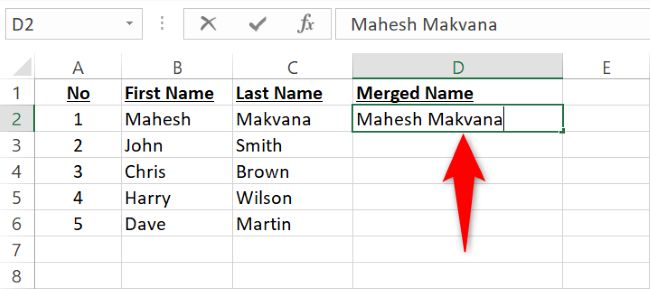
To use start using Flash Fill, in your spreadsheet, select the first cell where you want to display the combined names. In this cell, type the first and last names together as you'd like them to appear.
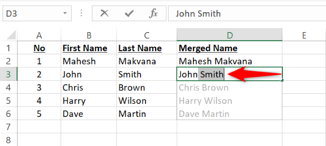
Go down a row and start typing the first and last name for your second record. As soon as you begin typing, Flash Fill will sense the pattern and fill all your records in gray color. To confirm you want these cells filled, press Enter on your keyboard.
If a Flash Fill prompt doesn't appear, use the Ctrl+E shortcut to force a Flash Fill.
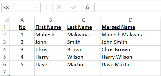
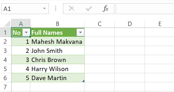
And that's it. Excel has automatically merged the first and last names for all your records.
Method 2: Use the & (Ampersand) Symbol
If you prefer to use an Excel formula to combine names, a simple method for bringing multiple cells' content into a single cell is to use the & (ampersand) operator. This operator combines the content of your specified cells, allowing you to merge all the cell data you want.
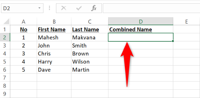
To use this method, in your spreadsheet, select the cell where you want to see the merged names.
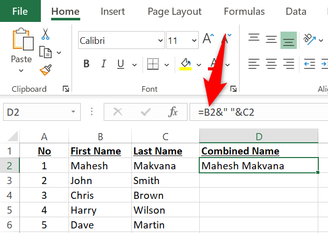
In the selected cell, type the following formula and press Enter. Here, replace B2 with the cell containing the first name and C2 with the cell that has the last name.
=B2&" "&C2
Note that we've added a space enclosed with double quotes so that there's a space between the first and the last name in the resulting cell.
In your selected cell, you'll see the first and last names combined.
To copy this formula for all your records, from the bottom-right corner of the cell where you've entered the formula, click and drag downwards covering all your records.
If you have a middle name or initial in a separate column and you'd like to merge that as well, add that cell as an argument to the formula. Here, we'll combine the contents of the cell B2 , C2 , and D2 (in that order), with each cell content separated by a space.
=B2&" "&C2&" "&D2
Alternatively, if you want to combine names so that the last name appears first followed by a comma, use a formula like this.
=D2&", "&B2&" "&C2
Method 3: Use the CONCAT Function
Excel's CONCAT function works just like the & operator and lets you combine multiple cells' content into a single cell. Using a function instead of an operator can sometimes make your formula easier for others to read and understand.
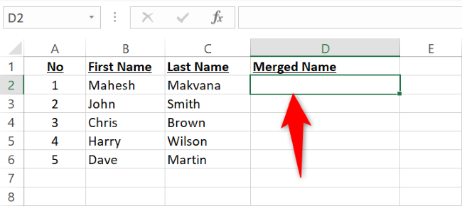
To merge your first and last names with CONCAT, in your spreadsheet, select the cell where you'd like to see the combined names.
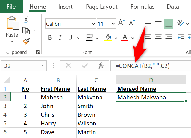
In the selected cell, enter the following function and press Enter. In this function, replace B2 with your cell that has the first name and C2 with the cell that contains the last name. Note that we've separated the first and the last name with a space in this function.
=CONCAT(B2," ",C2)
Once you press Enter, in your selected cell, you'll see both your names merged. You can copy the function for all your records by dragging downwards from the bottom-right corner of the cell where the function exists.
If you'd like to merge the middle name or initial as well, use the function as follows. Here, C2 denotes the middle name cell, while D2 contains the last name.
=CONCAT(B2," ",C2," ",D2)
If, instead, you want the last name to come first, try changing around the formula and inserting a comma like this:
=CONCAT(D2,", ",B2," ",C2)
And that's it.
Method 4: Use the TEXTJOIN Function
With the TEXTJOIN function, you can combine your names using your specified delimiter. This function also offers the option to ignore empty cells. You'll find it a little more complicated to use than CONCAT, but it's also a more powerful function.
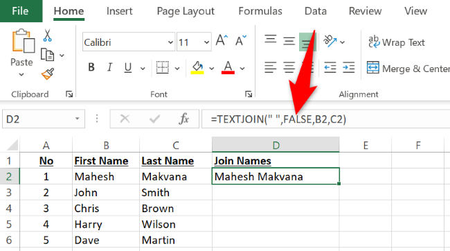
To use TEXTJOIN, in your spreadsheet, click the cell where you want to display the merged names. Then, type the following function in the cell. Here, replace B2 with the cell that has the first name and C2 with the cell containing the last name. To ignore empty cells, change FALSE to TRUE .
=TEXTJOIN(" ",FALSE,B2,C2)
If your dataset has first name, middle name, and last name in the B2 , C2 , and D2 cells, respectively, then you can join them using the following function:
=TEXTJOIN(" ",FALSE,B2,C2,D2)
Method 5: Use Power Query
Power Query is an Excel feature that helps you combine data from multiple worksheets and workbooks. You can use this option to merge your columns as well.
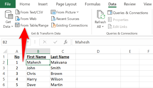
To use this method, first, click a cell in your dataset. Then, from Excel's ribbon at the top, select Data > From Table/Range.
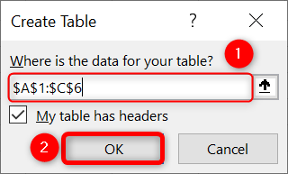
In the "Create Table" box, ensure the correct dataset range is specified. If your dataset has column headers, enable the "My Table Has Headers" option. Then, select "OK."
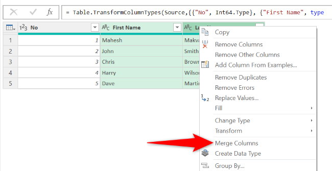
A "Power Query Editor" window will open. Here, hold down Ctrl (Windows) or Command (Mac) key and select your first name and last name columns. Then, right-click either column and choose "Merge Columns."
On the "Merge Columns" window, click the "Separator" drop-down menu and choose "Space." Optionally, in the "New Column Name" field, enter the name of the column that'll have your merged names. Then, select "OK."
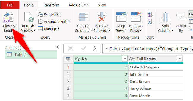
In the "Power Query Editor" window's top-left corner, click "Close & Load."
In your workbook, Power Query has added a new worksheet that contains your merged names.
You now have a spreadsheet complete with readable full names for each entry. If you're entering a lot of names and other data, learn the best Excel functions for data entry.


