Working with arrays, or adjacent cell ranges, in Microsoft Excel can be challenging at times. If you'd like to combine, reshape, or resize an array, you can choose from a collection of functions that can cover many situations.
These 11 functions are new to Excel as of August 2022. They're rolling out to Excel users over time beginning with Office Insiders.
Combine Arrays
Combining data in a spreadsheet can be difficult. With the VSTACK and HSTACK functions, you can stack arrays vertically and horizontally.
The syntax for each function is the same as
VSTACK(array1, array2,...)
and
HSTACK(array1, array2,...)
with only one required array and others optional.
To combine the arrays in cells B2 through F3 and H2 through L3 vertically, use this formula for the VSTACK function:
=VSTACK(B2:F3,H2:L3)
To combine those same arrays horizontally instead, use this formula for the HSTACK function:
=HSTACK(B2:F3,H2:L3)
Reshape Arrays
If it's not combining arrays that you want to do but reshaping them instead, there are four functions you can use.
Convert an Array to a Row or Column
First, the TOROW and TOCOL functions let you shape the array as a row or a column. The syntax for each is TOROW(array, ignore, by_column) and TOCOL(array, ignore, by_column).
- Ignore: To ignore certain types of data, enter 1 for blanks, 2 for errors, or 3 for blanks and errors. The default is 0 to ignore no values.
- By_column: Use this argument to scan the array by column using TRUE. If no argument is included, FALSE is the default, which scans the array by row. This determines how the values are ordered.
To convert the array B2 through F3 to a row, use this formula with the TOROW function:
=TOROW(B2:F3)
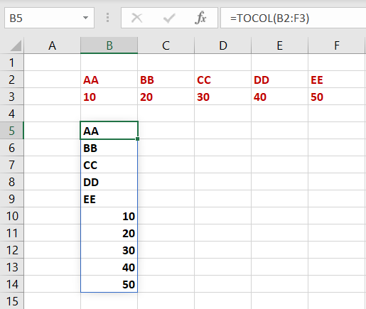
To convert that same array to a column instead, use the TOCOL function with this formula:
=TOCOL(B2:F3)
Convert a Row or Column to an Array
To do the opposite of the above and convert a row or column to an array, you can use WRAPROWS and WRAPCOLS. The syntax for each is WRAPROWS(reference, wrap_count, pad) and WRAPCOLS(reference, wrap_count, pad) with the reference being a group of cells.
- Wrap_count: The number of values for each row or column.
- Pad: The value to display for the pad (empty cell).
To convert the cells B2 through K2 to a two-dimensional array by wrapping rows, use the WRAPROWS function. With this formula, the cells are wrapped using three values per row with "empty" as the pad.
=WRAPROWS(B2:K2,3,"empty")
To convert the same cells into a two-dimensional array by wrapping columns, use the WRAPCOLS function. With this formula, the cells are wrapped using three values per column with "empty" as the pad.
=WRAPCOLS(B2:K2,3,"empty")
Resize Arrays
Maybe you want to adjust the size of an array by adding some data or dropping unnecessary cells. There are five functions to help you do this depending on the result you want.
Take or Drop Rows or Columns
With the TAKE function, you keep the number of rows or columns you specify. With the DROP function, you do the opposite and remove the number of rows or columns you specify. You'll use positive numbers to take or drop from the start of the array and negative numbers to take or drop from the end.
The syntax for each is TAKE(array, rows, columns) and DROP(array, rows, columns) where you need at least one of the second two arguments; rows or columns.
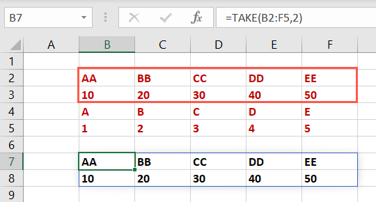
To keep the first two rows in the array B2 through F5, use TAKE with the rows argument. Here's the formula:
=TAKE(B2:F5,2)
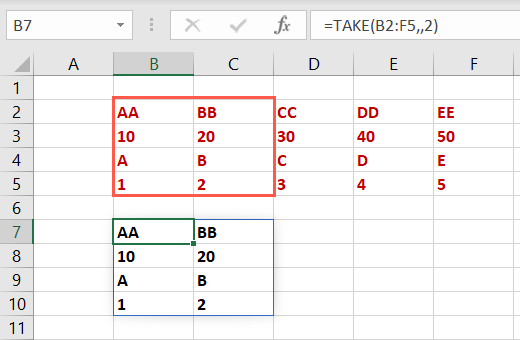
To keep the first two columns in that same array, use the columns argument instead:
=TAKE(B2:F5,,2)
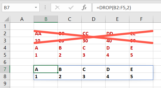
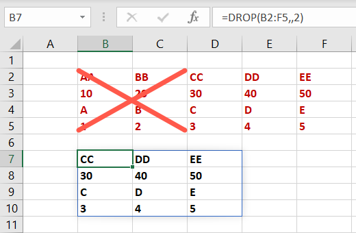
To remove the first two rows in the array B2 through F5, use DROP with the rows argument and this formula:
=DROP(B2:F5,2)
To remove the first two columns in that same array, use the columns argument instead and this formula:
=DROP(B2:F5,,2)
Keep a Certain Number of Rows or Columns
To select the exact row and column numbers you want to keep from an array, you'd use the CHOOSEROWS and CHOOSECOLS functions.
The syntax for each is CHOOSEROWS(array, row_num1, row_num2,...) and CHOOSECOLS(array, column_num1, column_num2,...) where the first two arguments are required. You can add more row and column numbers if you like.
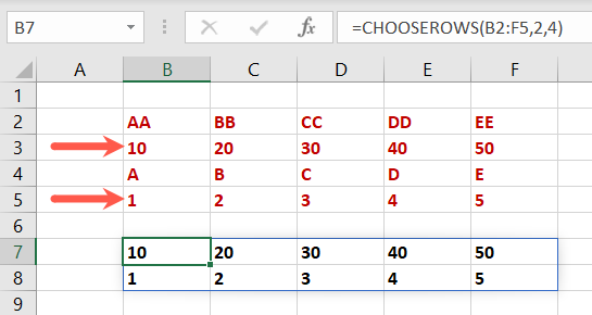
To return rows 2 and 4 from the array B2 through F5, you'd use the CHOOSEROWS function and this formula:
=CHOOSEROWS(B2:F5,2,4)
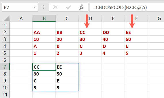
To return columns 3 and 5 from the same array, you'd use the CHOOSECOLS function with this formula:
=CHOOSECOLS(B2:F5,3,5)
Remember to use the row or column numbers for the array, not for the sheet.
Expand an Array to Specific Dimensions
Maybe you plan to add more data to your array, so you want to make it a specific size to add a border or use conditional formatting. With the EXPAND function, you enter the number of rows and columns your array should cover.
The syntax for the function is EXPAND(array, rows, columns, pad) where a missing rows or columns argument means those will not expand. Optionally, you can include the pad value for the empty cells.
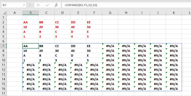
To expand the array B2 through F5 to cover 10 rows and 10 columns, you'd use this formula:
=EXPAND(B2:F5,10,10)
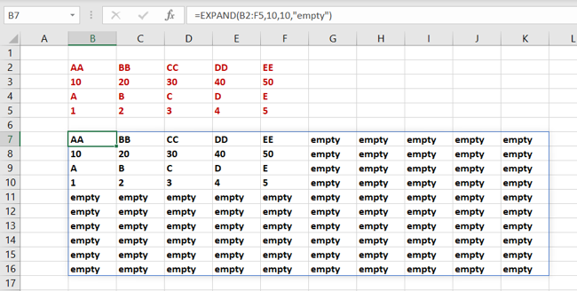
To expand that same array to the same dimensions and include the pad "empty," use this formula:
=EXPAND(B2:F5,10,10,"empty")
Although the pad argument is optional, you may prefer it over seeing an error as shown above.
These 11 functions give you more control than ever over your arrays in Microsoft Excel. Give them a try and see if they accomplish what you need.


