An easy way to make numbers stand out in Google Sheets is with conditional formatting. You can automatically apply formatting like a bold font or cell color when certain values meet your criteria.

One thing that makes conditional formatting a great option is that when you make edits to your sheet, that formatting automatically applies. So as your values change, you can see those numbers pop without any extra work.

We've shown you how to use conditional formatting based on date and how to use it for certain text. So let's get back to the most basic usage of the feature and automatically highlight values with it.

Set Up a Conditional Formatting Rule

Visit Google Sheets, sign in, open the workbook you want to use, and choose a sheet. Any rules you set up apply only to the current spreadsheet.

Related: How to Highlight a Row in Google Sheets Using Conditional Formatting

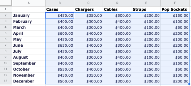
Select the cells you want to apply the conditional formatting rule to by dragging through adjacent cells or holding Ctrl (Windows) or Command (Mac) as you select nonadjacent cells.

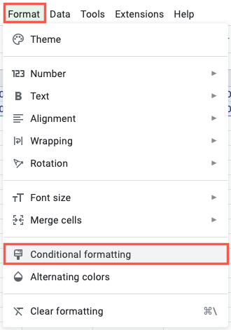
Go to the Format tab and choose "Conditional Formatting."

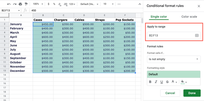
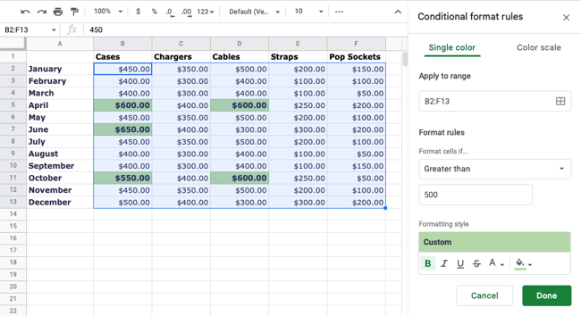
This opens a sidebar on the right for you to set up a rule. Select the Single Color tab at the top and confirm the cells in the Apply to Range box.

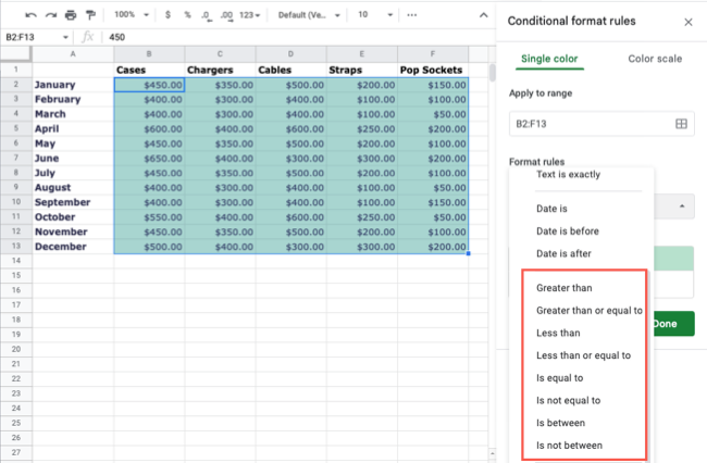
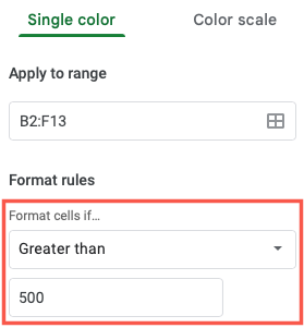
Next, pick the criteria you want to use in the Format Cells If drop-down box. You'll see eight options for numbers like greater than, less than, equal to, not equal to, and between.

As an example, we'll choose Greater Than to highlight sales higher than $500. After you pick the criteria, you'll add the corresponding value(s) in the box beneath.

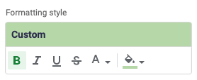
Now you can pick the Formatting Style using things like bold, italics, or underline for the font or a fill color for the cells. You can also use a combination of styles if you like. So, you can pick both a bold font and a green cell color.

As you select the formatting, you'll see your sheet update for a nice preview of your selection. This lets you make adjustments before you save the rule. When you're happy with the highlighting, click "Done" to apply the rule.

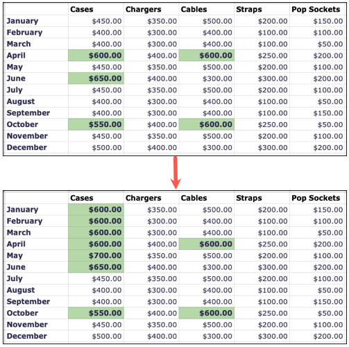
You should see the cells that meet your criteria highlighted. And, if you make any changes to those cells that affect the criteria, they automatically update.

Conditional Formatting Examples

Let's look at more example uses for conditional formatting based on values.

Related: How to Highlight Duplicates in Google Sheets

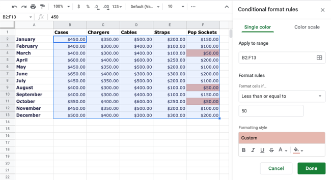
You can use the Less Than or Equal To criteria to highlight the smallest values in the range. Here, we can see our lowest sales, those equal to or less than 50.

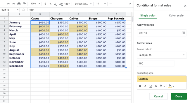
Maybe you want to see specific values. Here, we want to see all sales that are exactly $400 using the Is Equal To criteria with 400 as the matching value.

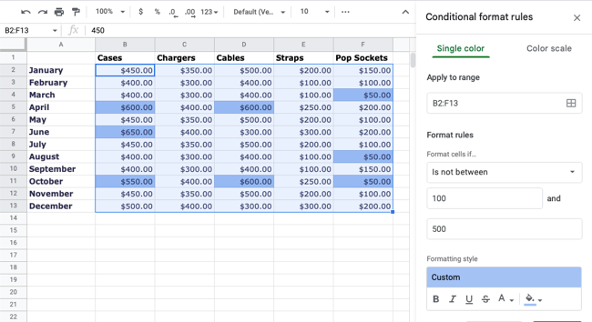
You can use the Is Not Between criteria to spot those numbers outside of a range. Here, we enter 100 and 500 to find those values not between those numbers. This lets us see our highest and lowest sales at the same time.

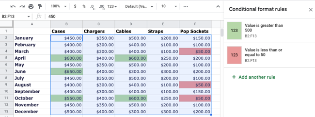
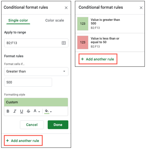
If you want to set up more than one conditional formatting rule for your sheet, you can do that too. Here, we have our highest values with a green fill color and our lowest with red.

To add more rules, select "Add Another Rule" at the bottom of the sidebar for the current rule or when you first open it.

Edit or Remove a Conditional Formatting Rule

After you set up your rule, you can make changes to it or delete it completely if you like.

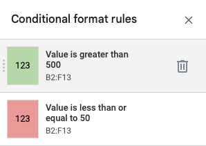
Head back to Format > Conditional Formatting to open the sidebar. You'll see all rules you've set up for that sheet.

• To make a change, simply select the rule, edit what you want, and select "Done" to save it.
• To remove a rule, hover your cursor over it in the list and click the trash can icon that displays.

Conditional formatting in Google Sheets gives you a terrific way to see the values you want at a glance. You can make negative numbers pop or try the color scale option.