Lookup functions in Microsoft Excel are ideal for finding what you need when you have a large amount of data. There are three common ways to do this; INDEX and MATCH, VLOOKUP, and XLOOKUP. But what's the difference?
INDEX and MATCH, VLOOKUP, and XLOOKUP each serve the purpose of looking up data and returning a result. They each work a bit differently and require a specific syntax for the formula. When should you use which? Which is better? Let's take a look so you know the best option for you.
Using INDEX and MATCH
Obviously, the INDEX and MATCH combination is a mixture of the two named functions. You can take a look at our how-tos for the INDEX function and MATCH function for specific details on using them individually.
To use this duo, the syntax for each is
INDEX(array, row_number, column_number)
and
MATCH(value, array, match_type)
.
When you combine the two, you'll have a syntax like this:
INDEX(return_array, MATCH(lookup_value, lookup_array))
in its most basic form. It's easiest to look at some examples.
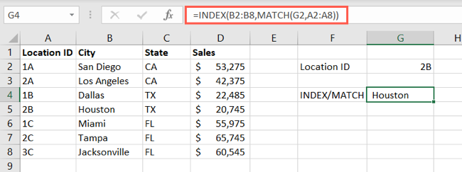
To find a value in cell G2 in the range A2 through A8 and provide the matching result in the range B2 through B8, you would use this formula:
=INDEX(B2:B8,MATCH(G2,A2:A8))
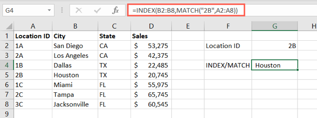
If you prefer to insert the value you want to find instead of using the cell reference, the formula looks like this where 2B is the lookup value:
=INDEX(B2:B8,MATCH("2B",A2:A8))
Our result is Houston for both formulas.
We also have a tutorial that goes into detail on using INDEX and MATCH should that be your choice.
Using VLOOKUP
VLOOKUP has been a popular reference function in Excel for some time. The V stands for Vertical, so with VLOOKUP, you're doing a vertical lookup and it's from left to right.
The syntax is VLOOKUP(lookup_value, lookup_array, column_number, range_lookup) with the last argument optional as True (approximate match) or False (exact match).
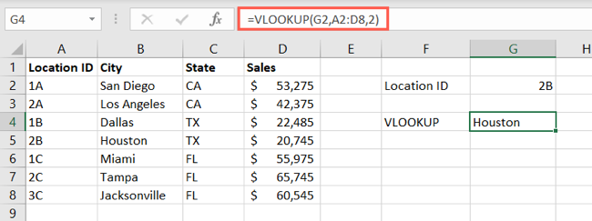
Using the same data as that for INDEX and MATCH, we'll look up the value in cell G2 in the range A2 through D8 and return the value in the second column that matches. You'd use this formula:
=VLOOKUP(G2,A2:D8,2)
As you can see, the result using VLOOKUP is the same as using INDEX and MATCH, Houston. The difference is that VLOOKUP uses a much simpler formula. For more details on VLOOKUP, check out our how-to.
So why would anyone use INDEX and MATCH instead of VLOOKUP? The answer is because VLOOKUP only works when your lookup value is to the left of the return value you want.
If we did the reverse and wanted to look up a value in the fourth column and return the matching value in the second column, we would not receive the result we want and may even receive an error. As Microsoft writes:
Remember that the lookup value should always be in the first column in the range for VLOOKUP to work correctly. For example, if your lookup value is in cell C2 then your range should start with C.
INDEX and MATCH covers the entire cell range or array making it a more robust lookup option even if the formula is a bit more complicated.
Using XLOOKUP
XLOOKUP is a reference function that arrived in Excel after VLOOKUP and the counterpart HLOOKUP (horizontal lookup). The difference between XLOOKUP and VLOOKUP is that XLOOKUP works no matter where the lookup and return values reside in your cell range or array.
The syntax is XLOOKUP(lookup_value, lookup_array, return_array, not_found, match_mode, search_mode). The first three arguments are required and are similar to that in the VLOOKUP function. XLOOKUP offers three optional arguments at the end for giving a text result if the value isn't found, a mode for the type of match, and a mode for how to perform the search.
For the purpose of this article, we'll concentrate on the first three required arguments.
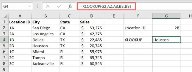
Back to our cell range from earlier, we'll look up the value in G2 in the range A2 through A8 and return the matching value from the range B2 through B8 with this formula:
=XLOOKUP(G2,A2:A8,B2:B8)
And like with INDEX and MATCH as well as VLOOKUP, our formula returned Houston.
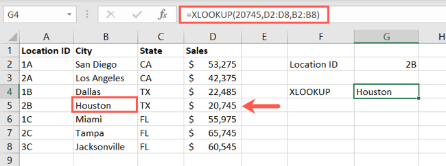
We can also use a value in the fourth column as the lookup value and receive the correct result in the second column:
=XLOOKUP(20745,D2:D8,B2:B8)
With this in mind, you can see that XLOOKUP is a better option than VLOOKUP simply because you can arrange your data any way you like and still receive your desired result. For a full tutorial on XLOOKUP, head over to our how-to.
So now you're wondering, should I use XLOOKUP or INDEX and MATCH, right? Here are some things to consider.
Which Is Better?
If you already use the INDEX and MATCH functions separately and have used them together to lookup values, then you may be more familiar with how they work. By all means, if it's not broken, don't fix it, and keep using what makes you comfortable.
And of course, if your data is structured to work with VLOOKUP and you've used that function for years, you can continue using it or make the easy transition to XLOOKUP leaving INDEX and MATCH in the dust.
If you want to a simple, easy-to-build formula in any direction, XLOOKUP is the way to go and can replace INDEX and MATCH. You don't have to worry about combining arguments from two functions into one or rearranging your data.
One last consideration, XLOOKUP does offer those three optional arguments which may come in handy for your needs.
Over to you! Which lookup option will you use in Microsoft Excel? Or maybe, you'll use all three depending on your needs? No matter what, it's nice to have options!


