Quick Links
Using a pivot table, you can analyze large amounts of data easily. But as we all know, data can and often does change. To make sure that your data is current, here's how to refresh a pivot table in Excel.
Whether the data in your pivot table comes from an external source or the same workbook, you can update it manually or automatically. You can also adjust a setting so that the formatting doesn't change when you update the table.
Refresh a Pivot Table Manually
If you would prefer to update your pivot table manually when needed, start by selecting the table.
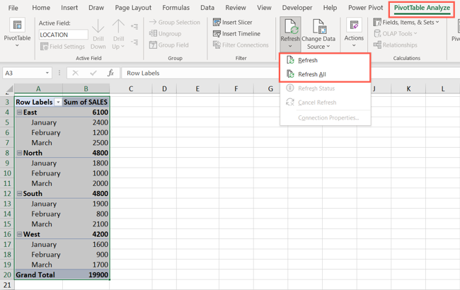
Go to the PivotTable Analyze tab that appears. Click the Refresh drop-down arrow in the Data section of the ribbon.
To refresh the selected pivot table, choose "Refresh." To refresh all pivot tables in your workbook, choose "Refresh All."
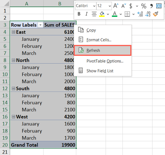
Alternatively, you can right-click the pivot table and choose "Refresh" in the shortcut menu.
If the update takes a bit of time, you can select Refresh > Refresh Status to see the progress. To cancel, choose Refresh > Cancel Refresh.
Refresh a Pivot Table Automatically
Maybe you'd rather that your pivot table update each time you open the workbook. This is a good way to always have refreshed data and saves you from remembering to manually update the table.
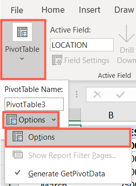
Select the pivot table and go to the PivotTable Analyze tab. On the left side, use the PivotTable drop-down arrow and click Options > Options.
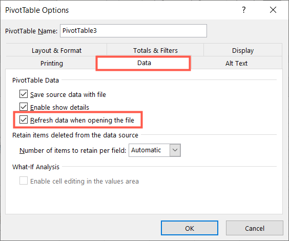
In the PivotTable Options window, select the Data tab. Then, check the box for Refresh Data When Opening the File. Click "OK."
Prevent Formatting Changes Upon Update
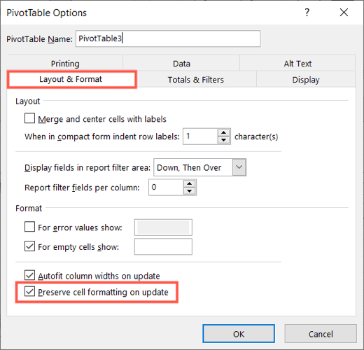
Sometimes the data that gets updated is wider than your column width or longer than your row height. If you want to retain the formatting for your columns and rows when you refresh a pivot table, it's a simple setting.
Select the pivot table and go to the PivotTable Analyze tab. On the left side, use the PivotTable drop-down arrow and then click Options > Options.
In the PivotTable Options window, select the Layout & Format tab. Then, check the box for Preserve Cell Formatting on Update. Optionally, you can check the box directly above for Autofit Column Widths on Update. Click "OK."
Keep your data current and up to date by refreshing your pivot table in Excel, either manually or automatically.


