Quick Links
Using slicers, you can filter data and always see what's being filtered in your Microsoft Excel spreadsheets. You can add a slicer for each field you want to filter, and we'll show you how to do that.
What Is a Slicer in Excel?
A slicer is basically an on-screen tool that you can use to filter data in your spreadsheet's tables. For example, if you have a data table containing various countries, you can create a slicer that only displays records where the country is the USA.
This slicer always remains on your screen, so you or anyone else who opens the spreadsheet knows exactly how your data is filtered. Slicers are customizable and you can apply different color schemes and sizes to them, as we'll explain below.
Make a Slicer in Microsoft Excel
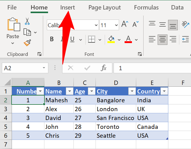
To start the slicer-making process, first, open your spreadsheet with Microsoft Excel. Then click the table in which you want to filter data using a slicer.
While your table is selected, in Excel's ribbon at the top, click the "Insert" tab.
On the "Insert" tab, in the "Filters" section, click "Slicer" to add a slicer.
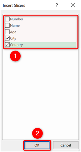
You'll see an "Insert Slicers" window displaying your table's fields. Here, choose the fields which you want to filter using a slicer, then click "OK" at the bottom.
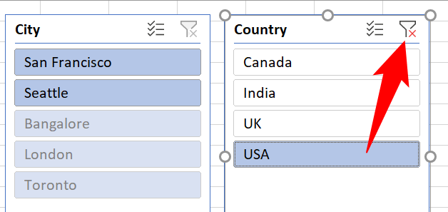
Excel will add a slicer for each selected field. To start filtering your data, select an option in one of these slicers and the data in your table will adjust accordingly.
If you'd like to apply multiple filters in a single slicer, you can select multiple options by holding down the Ctrl (Windows) or Command (Mac) key.
To reset a slicer's filter, then in that slicer's top-right corner, click the "Clear Filter" option.
And that's it.
Customize a Slicer in Microsoft Excel
Slicers can be customized to use a specified color or size. You can also drag and drop slicers to place them wherever you want on your screen.
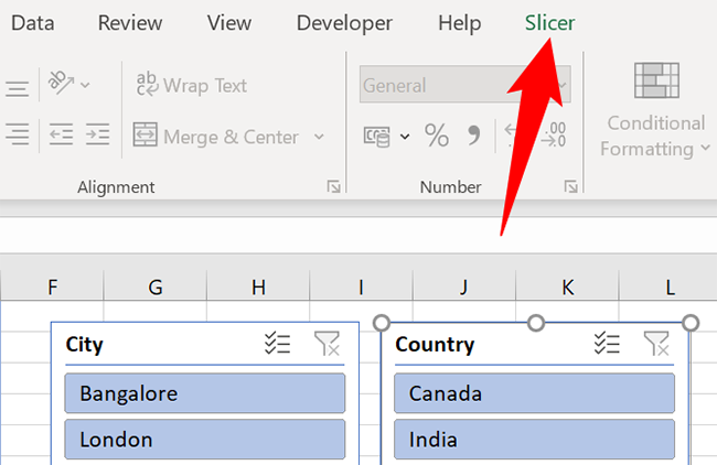
To access your slicer's personalization options, first, choose a slicer in your spreadsheet. Then in Excel's ribbon at the top, click the "Slicer" tab to access all customization options.
You'll now find various options to change how your slicers look in your spreadsheet. For example, to change your slicer's color, you can pick a new color scheme from the "Slicer Styles" section.
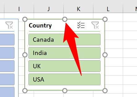
Similarly, to resize your slicer, you can use the "Height" and "Width" boxes at the top. Another way to resize a slicer is to click it and then drag its dot icons.
Once you've customized your slicers, don't forget to save your spreadsheet to keep your changes. And you're all set.
While you're at it, check out other ways to sort and filter data in Excel. You might find these helpful for your spreadsheet tasks.


