Many times, the text in your spreadsheet is just as important as the numbers, or maybe more depending on your data. If you want to make certain text stand out, you can automatically highlight it in Google Sheets.
You may have a sheet containing customer names, product details, student grades, or business locations. With conditional formatting, you can automatically highlight the text you need so that you can spot it quickly.
Set Up Conditional Formatting for Text in Google Sheets
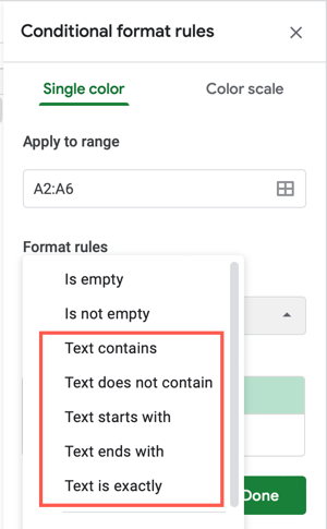
Google Sheets offers several ways to automatically highlight the text you want. Your options are:
- Text contains
- Text does not contain
- Text starts with
- Text ends with
- Text is exactly
You can choose the option that fits your data.
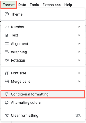
To apply the conditional formatting, select the cells you want to format, go to the Format tab, and choose "Conditional Formatting."
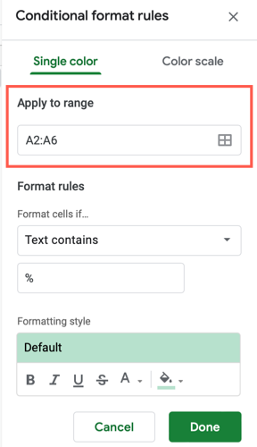
Use the Single Color tab at the top of the sidebar that appears. Confirm the cell range in the Apply to Range box or add another range if you like.
Under Format Rules, use the Format Cells If drop-down box to choose one of the above text options. In the subsequent cell, enter the text to look for.
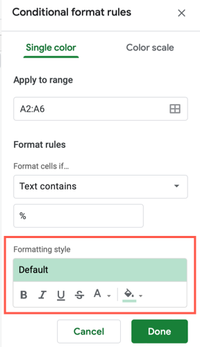
Set up the font or cell highlighting in the Formatting Style section and click "Done" to apply the conditional formatting rule.
Let's look at some examples.
Text Contains or Does Not Contain
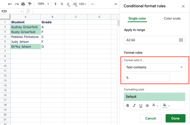
Maybe you imported data that contains random characters like percent signs. You want to highlight the cells so that you can correct that data. For this situation, you can use Text Contains for the rule.
Follow the steps above to select the cells and open the Conditional Formatting sidebar. Choose "Text Contains" in the Format Cells If drop-down box and enter the percent sign in the box below it.
Pick the formatting you want to use, then click "Done," and you should see all the cells highlighted that contain the character you want to correct.
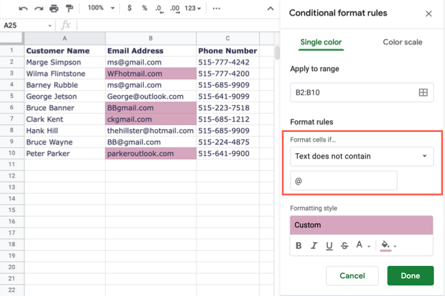
Alternatively, maybe you want to review a sheet for email addresses and highlight those that do not contain the @ (at) symbol so you can fix them. For this scenario, you would use Text Does Not Contain for the rule.
Select the cells and open the sidebar. Pick "Text Does Not Contain" in the Format Cells If drop-down box and enter the @ (at) symbol in the box below it.
When you set up the formatting and click "Done," you should see the cells highlighted that are missing that symbol you need for an email address.
Text Starts or Ends With
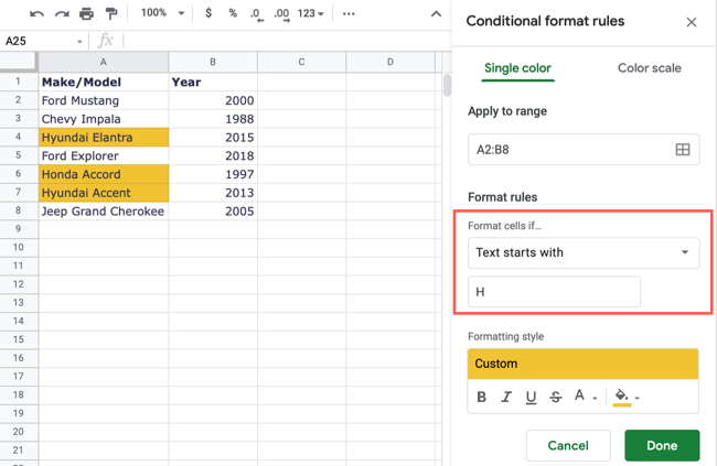
You can use entire words, a set of letters, or even a single letter to find the text you need. Here, we have a list of vehicles and we want to highlight all of the Honda and Hyundai models. For this rule, you can use the Text Starts With option.
Select the cells and open the sidebar to create the rule. Pick "Text Starts With" in the Format Cells If drop-down box and enter the letter H in the box below it.
Choose the format for the cells or text and click "Done" to highlight all the Honda and Hyundai vehicles in the list.
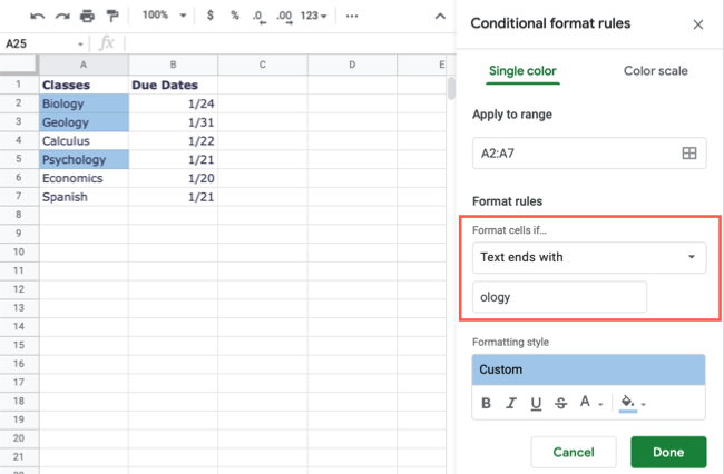
For an example using a set of letters, we'll highlight all science classes that end in "ology" using the Text Ends With option.
Select the cells and open the sidebar to create the rule. Pick "Text Ends With" in the Format Cells If drop-down box and enter "ology" in the box below it.
Choose the format for the cells or text and click "Done" to highlight all the science classes in the list.
Text Is Exactly
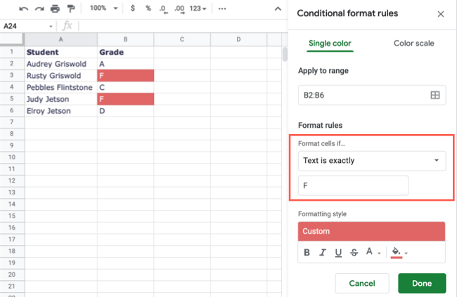
For our final example, we have a sheet of student names and grades. We want to apply conditional formatting so that when a student receives a grade of F, that grade is highlighted. Here, you would use the Text Is Exactly option for the rule.
Select the cells and open the sidebar. Pick "Text Is Exactly" in the Format Cells If drop-down box and enter the letter F in the box below it.
Choose the format and click "Done" to highlight all letter F grades.
When you want to highlight specific text in your Google Sheet, conditional formatting provides you with several options to find the exact text you need.
For more ways to use conditional formatting in Google Sheets, take a look at how to highlight blanks or errors or how to apply a color scale based on value.

