Quick Links
If you use Microsoft Excel for accounting purposes, you might want to use the accounting number format for your numbers. There are multiple ways to apply this formatting, and we'll show how.
What Is the Accounting Number Format?
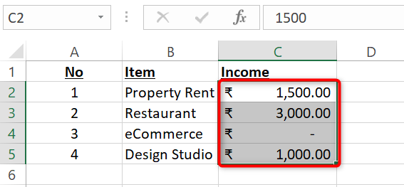
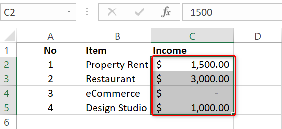
At first glance, the accounting number format looks like the currency format. However, there are a few differences between the two.
Those differences are:
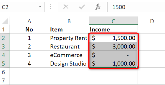
- Currency Sign: The accounting number format places the currency sign to the extreme left of the cell.
- Zeros as Dashes: Your zeros are displayed as dashes in this number format.
-
Negatives in Parentheses: The negative numbers are displayed in
()
All of the methods below let you apply the same accounting number format to your numbers, so use whatever method you find easier to do.
Apply the Accounting Number Format With a Ribbon Option
Excel has an option in its ribbon to help you quickly use the accounting number format in your spreadsheets.
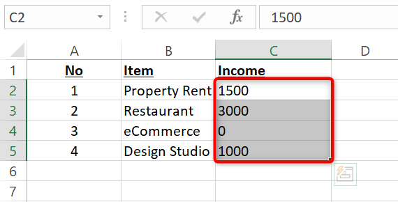
To use it, first, open your spreadsheet with Microsoft Excel. In your spreadsheet, select the cells containing the numbers that you want to turn into accounting numbers.
In Excel's ribbon at the top, click the "Home" tab.
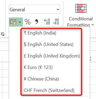
On the "Home" tab, in the "Number" section, click the down-arrow icon next to the "Accounting Number Format" option.
In the menu that opens, select the currency for your numbers.
And your selected numbers now use the accounting number format.
You're all set.
Apply the Accounting Number Format With a Drop-Down Menu
Another way to apply the accounting number format is to use the number formatting drop-down menu.
To use this method, open your spreadsheet with Microsoft Excel. Then select the cells with numbers in them.
In Excel's ribbon at the top, click the "Home" tab.
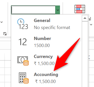
On the "Home" tab, in the "Number" section, click the drop-down menu.
From the drop-down menu, choose "Accounting."
And all your selected numbers are now in the accounting number format.
That's it.
Use Accounting Numbers With the Format Cells Window
The third way to use the accounting number format in Excel is by opening the Format Cells window.
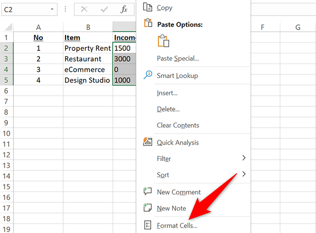
To do that, open your spreadsheet and select the cells with the numbers in them. Right-click one of these cells and select "Format Cells" from the menu.
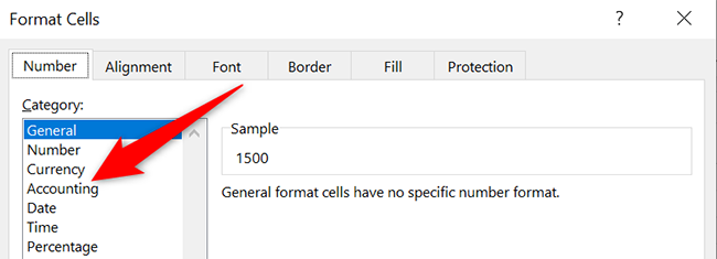
A "Format Cells" window will open. Here, from the "Category" list on the left, select "Accounting."
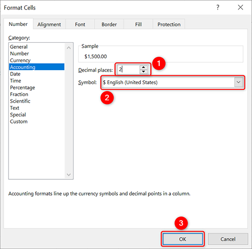
In the pane on the right, specify decimal points for your numbers using the "Decimal Places" option. Then, choose a currency from the "Symbol" drop-down menu.
Finally, click "OK" at the bottom of the window.
Your chosen cells are now formatted in the accounting number format.
You're now ready for your accounting tasks in your Excel spreadsheets.
Does Excel remove the zero from the beginning of your numbers? There's a way to make it keep those zeros.


