If you have data in a spreadsheet that you want to review quickly, having differences highlighted automatically can save you time. You might not realize it, but Microsoft Excel has a built-in feature for easily displaying row differences.

Once you locate the differing data, you can also apply formatting to keep those differences highlighted. Then, get to work on updating, correcting, or analyzing the data in your spreadsheet.

Find Row Differences in Excel

The first step in locating differences in your data is to select the cells. Drag your cursor through a group of cells or adjacent rows.

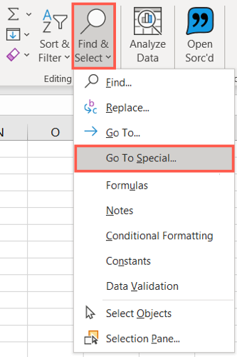
Next, head to the Home tab and the Editing section of the ribbon. Click "Find & Select" and pick "Go To Special" in the drop-down list.

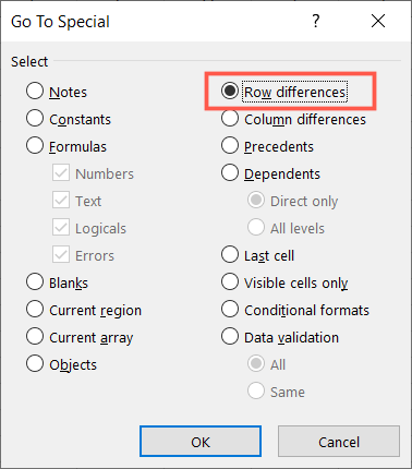
In the window that pops open, choose "Row Differences" and click "OK."

The window will automatically close, and you'll see the differences in your rows highlighted.

The Active Cell and Row Differences

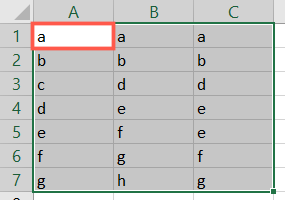
It's essential to know that the differences highlighted are based on the active cell. As you can see in the screenshot below, the active cell is A1 because it's white. This is the first cell that we selected when we dragged through the range. The same rule applies if you select rows instead of a cell range.

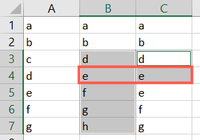
This means that the data in the subsequent rows that you see highlighted differs from that active cell's column. In the screenshot below, you can see that cells B4 and C4 are highlighted because they both differ from A4.

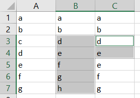
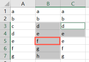
But in the following screenshot, only cell B5 is highlighted. This is because the data in C5 matches that in A5.

If you want to change the active cell, you can press Enter on Windows or Return on Mac with the Tab key to move to the cell that you want to make active. You can also start selecting the cell range with a different cell to make that one active. Just keep in mind that this affects the differences that display.

The key thing to remember here is that row differences are based on the active cell.

In the screenshots above, cell C3 became the active cell after applying row differences. You can still see the highlight indicator as a border.

Highlight Row Differences in Excel

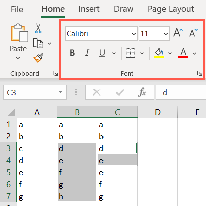
After you use the Go To Special feature above and see your row differences highlighted, you can stay on the Home tab and use a formatting option in the ribbon.

The Font section on the Home tab gives you options to change the text to bold, italics, or underline as well as adjust the font style, size, and color. Alternatively or in addition, you can select a fill color for the cells or apply a border.

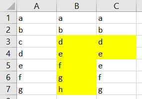
Once you apply your desired formatting to the cells, you can now travel about the sheet. The formatting that you manually applied will stick.

There are so many uses for Microsoft Excel that we end up with varieties of ways to accomplish tasks within it. So, if you're interested in the opposite of differences and want to catch duplicate data or simply remove duplicate rows in Excel, those are also easy tricks to learn.