Spotting things in a spreadsheet can be much quicker when you use colors that jump off the screen. With conditional formatting in Microsoft Excel, you can make finding blank cells or formula errors easier.

How to Automatically Highlight Blank Cells in Excel

When you have a spreadsheet full of data that you expect to fill every cell, you can easily overlook cells that are left empty. And a lack of data can be just as detrimental as incorrect data. Here's how to see blank cells by using conditional formatting.

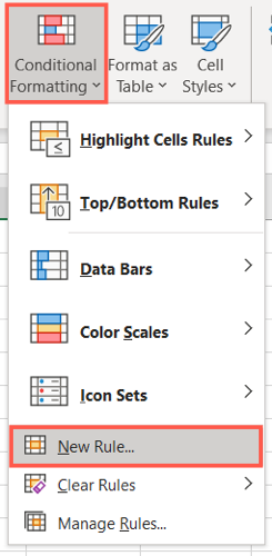
Open the sheet and select the cells where you want to apply the formatting. Head to the Home tab and click "Conditional Formatting" in the Styles group of the Ribbon. Choose "New Rule."

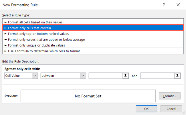
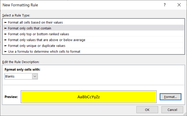
In the New Formatting Rule window that appears, pick "Format Only Cells That Contain" under Select the Rule Type at the top.

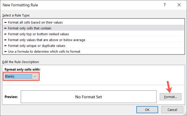
At the bottom, pick "Blanks" in the Format Only Cells With drop-down box. Then, click "Format" to the right of the preview to select how to format the blank cells.

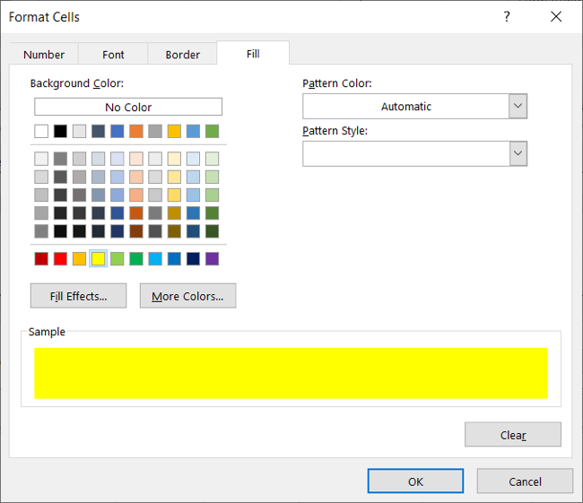
In the Format Cells window, use the tabs at the top for Font, Border, and Fill to choose your formatting. Click "OK." For our example, we'll use Fill to color our blank cells bright yellow.

You'll be back on the New Formatting Rule window, where you'll see a preview of the formatting for blank cells. If you're happy with it, click "OK" to apply the conditional formatting.

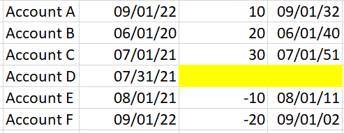
You should then see any empty cells in the range that you selected highlighted with the formatting that you picked.

Related: How to Check If a Cell Is Blank With ISBLANK in Excel

How to Automatically Highlight Errors in Excel

Even though Microsoft Excel does a decent job of shouting errors out to you, they might not be noticeable if you have a large sheet to scroll through. To make sure that you see the errors quickly, conditional formatting can save the day.

You'll actually follow the same process that you used in the previous section to highlight blanks, but with one difference.

Switch to the Home tab, click "Conditional Formatting," and then choose "New Rule."

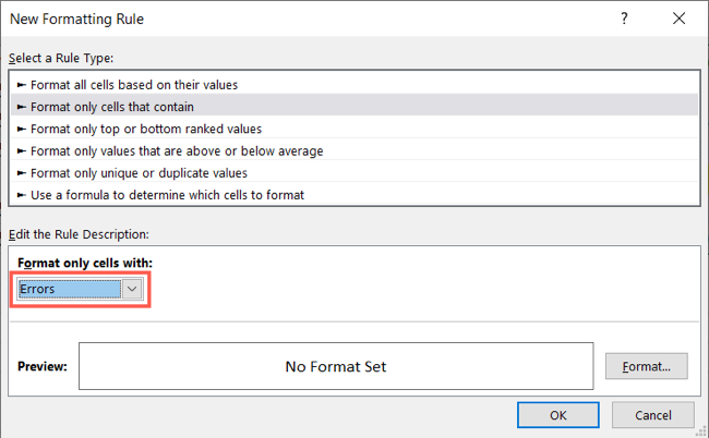
In the New Formatting Rule window, pick "Format Only Cells That Contain" at the top. But this time, pick "Errors" in the Format Only Cells With drop-down box at the bottom.

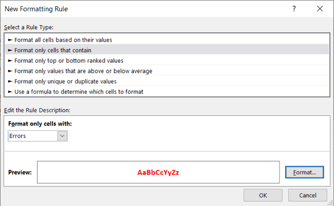
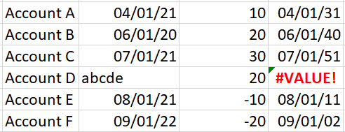
Then, click "Format" to choose the formatting. For this example, adjust the Font options to make the cells with errors bold and red. Click "OK" after you pick the formatting and "OK" again to apply the rule.

Now, those errors pop off the screen!

You can use this type of formatting in Microsoft Excel to do many other things as well. Check out how to use conditional formatting to highlight a row based on content or how to create a progress bar in Excel.