Quick Links
Key Takeaways
- Manually resize columns or rows in Google Sheets by dragging the border of the cell with your mouse or trackpad.
- Automatically resize columns or rows in Google Sheets by double-clicking the border to fit the largest cell's content.
- Use the column and row resizing tool in Google Sheets to resize to a specific size or automatically to fit the data.
When you open a new Google Sheets spreadsheet, the columns, rows, and individual cells you see will all be a certain size. If you want to see more data in each cell, you'll need to resize them. Here's how.
Manually Resizing a Column or Row in Google Sheets
One of the quickest ways to resize a column or row in Google Sheets is to use your mouse or trackpad to resize it manually. This involves dragging the column or row border to a new position, resizing it in the process.
To do this, open a Google Sheets spreadsheet containing your data. Below the formula bar, you'll see your column headers, initially ranging from A to Z. Likewise, row headers are seen on the left-hand side, initially ranging from 1 to 100.
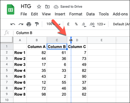
To resize either a row or column, hover over the column (A, B, etc.) or row (1, 2, etc.) header and move your mouse to the border. Your cursor should turn to an arrowhead, pointing in either direction.
Using your mouse or trackpad, drag the border to a new position, releasing it once the border is in place. A blue line will appear as the border is being moved, giving you a visual indication of the size of the new column or row.
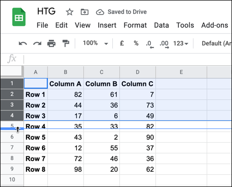
You can also complete this step for multiple columns or rows at once by first selecting them, then using your mouse or trackpad to resize the border on one of the columns or rows.
Google Sheets will treat the selected cells together, resizing them all to the same size.
Resizing Rows or Columns Automatically in Google Sheets
If the cells in your chosen row or column contain too much data, some of the information may be hidden from review (unless you wrap the text first).
To quickly resize these columns or rows to display this data without wrapping the cell text, you can use your mouse to resize it to fit. This will display all hidden text, resizing the column or row to match the size of the largest cell containing the most data.
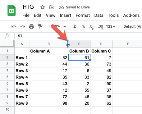
To do this, open your spreadsheet and hover over the column (starting with A, B, etc.) or row (starting with 1, 2, etc.) header labels. Move your cursor to hover over the border until the cursor changes to an arrowhead.
Once the arrowhead cursor is visible, double-click the border. This will force Google Sheets to resize it automatically to fit the content of the largest cell.
As with the manual method above, you can select multiple rows or columns to resize them at once. This will automatically resize each row or column to fit the largest cell's data.
Using the Resize Column or Row Tool in Google Sheets
The steps above allow you to resize columns and rows using your mouse or trackpad, but these methods don't offer a way to resize them to a set size. To do this, you'll need to use Google Sheets' column and row resizing tool.
To start, open your spreadsheet and select the header for your row (starting with 1, 2, etc.) or column (starting with A, B, etc.) to select it. You can also do this for multiple rows and columns at once by selecting them first.
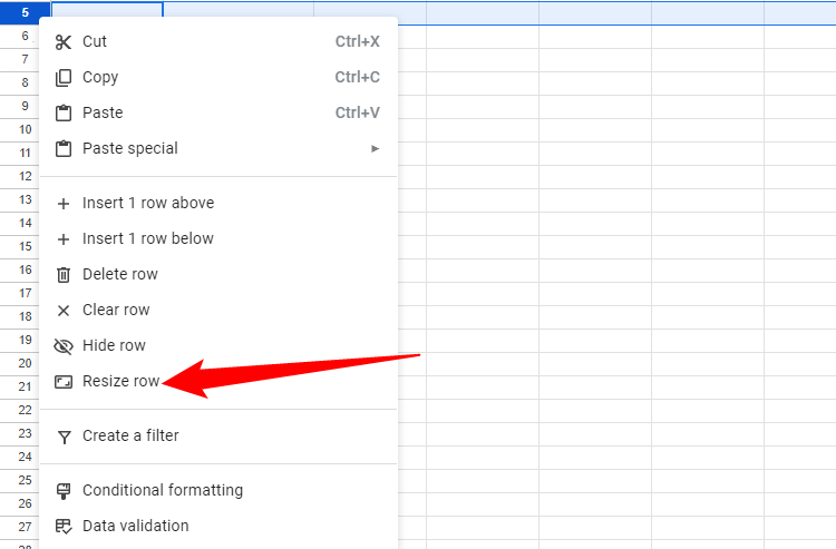
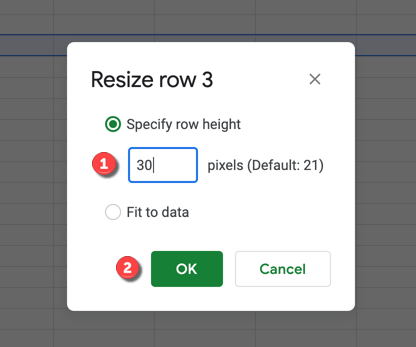
With the row or column you wish to resize selected, right-click the header label itself (eg. 1 or A). From the pop-up menu, click the "Resize The Column" or "Resize The Row" option.
In the "Resize" box for your row or column, enter a new size (in pixels) in the box provided to resize it. Alternatively, select the "Fix To Data" option to automatically resize the column or row to fit the largest cell's data.
Press "OK" to make the change once you're happy with the new sizing.
Once confirmed, the column or row will resize to match the size you selected. You can repeat this step for additional rows or columns.

