If you need to manipulate data in Google Sheets, the QUERY function can help! It brings powerful, database-style searching to your spreadsheet, so you can look up and filter your data in any format you like. We'll walk you through how to use it.
Using the QUERY Function
The QUERY function isn't too difficult to master if you've ever interacted with a database using SQL. The format of a typical QUERY function is similar to SQL and brings the power of database searches to Google Sheets.
The format of a formula that uses the QUERY function is
=QUERY(data, query, headers)
. You replace "data" with your cell range (for example, "A2:D12" or "A:D"), and "query" with your search query.
The optional "headers" argument sets the number of header rows to include at the top of your data range. If you have a header that spreads over two cells, like "First" in A1 and "Name" in A2, this would specify that QUERY use the contents of the first two rows as the combined header.
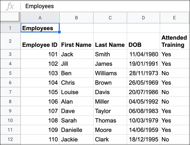
In the example below, a sheet (called "Staff List") of a Google Sheets spreadsheet includes a list of employees. It includes their names, employee ID numbers, birth dates, and whether they've attended their mandatory employee training session.
On a second sheet, you can use a QUERY formula to pull a list of all of employees who haven't attended the mandatory training session. This list will include employee ID numbers, first names, last names, and whether they attended the training session.
To do this with the data shown above, you could type
=QUERY('Staff List'!A2:E12, "SELECT A, B, C, E WHERE E = 'No'")
. This queries the data from range A2 to E12 on the "Staff List" sheet.
Like a typical SQL query, the QUERY function selects the columns to display (SELECT) and identifies the parameters for the search (WHERE). It returns columns A, B, C, and E, providing a list of all matching rows in which the value in column E ("Attended Training") is a text string containing "No."
As shown above, four employees from the initial list haven't attended a training session. The QUERY function provided this info, as well as matching columns to show their names and employee ID numbers in a separate list.
This example uses a very specific range of data. You could change this to query all the data in columns A to E. This would allow you to continue to add new employees to the list. The QUERY formula you used will also update automatically whenever you add new employees or when someone attends the training session.
The correct formula for this is
=QUERY('Staff List'!A2:E, "Select A, B, C, E WHERE E = 'No'")
. This formula ignores the initial "Employees" title in cell A1.
If you add an 11th employee who hasn't attended the training to the initial list, as shown below (Christine Smith), the QUERY formula updates, as well, and displays the new employee.
Advanced QUERY Formulas
The QUERY function is versatile. It allows you to use other logical operations (like AND and OR) or Google functions (like COUNT) as part of your search. You can also use comparison operators (greater than, less than, and so on) to find values between two figures.
Using Comparison Operators with QUERY
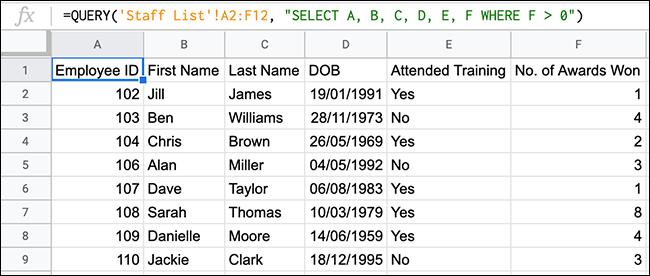
You can use QUERY with comparison operators (like less than, greater than, or equal to) to narrow down and filter data. To do this, we'll add an additional column (F) to our "Staff List" sheet with the number of awards each employee has won.
Using QUERY, we can search for all employees who have won at least one award. The format for this formula is
=QUERY('Staff List'!A2:F12, "SELECT A, B, C, D, E, F WHERE F > 0")
.
This uses a greater than comparison operator (>) to search for values above zero in column F.
The example above shows the QUERY function returned a list of eight employees who have won one or more awards. Out of 11 total employees, three have never won an award.
Using AND and OR with QUERY
Nested logical operator functions like AND and OR work well within a larger QUERY formula to add multiple search criteria to your formula.
A good way to test AND is to search for data between two dates. If we use our employee list example, we could list all employees born from 1980 to 1989.
This also takes advantage of comparison operators, like greater than or equal to (>=) and less than or equal to (<=).
The format for this formula is
=QUERY('Staff List'!A2:E12, "SELECT A, B, C, D, E WHERE D >= DATE '1980-1-1' and D <= DATE '1989-12-31'")
. This also uses an additional nested DATE function to parse date timestamps correctly, and looks for all birthdays between and equal to January 1, 1980, and December 31, 1989.
As shown above, three employees who were born in 1980, 1986, and 1983 meet these requirements.
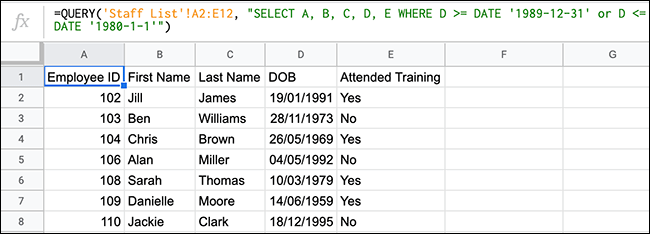
You can also use OR to produce similar results. If we use the same data, but switch the dates and use OR, we can exclude all employees who were born in the 1980s.
The format for this formula would be
=QUERY('Staff List'!A2:E12, "SELECT A, B, C, D, E WHERE D >= DATE '1989-12-31' or D <= DATE '1980-1-1'")
.
Of the original 10 employees, three were born in the 1980s. The example above shows the remaining seven, who were all born before or after the dates we excluded.
Using COUNT with QUERY
Rather than simply searching for and returning data, you can also mix QUERY with other functions, like COUNT, to manipulate data. Let's say we want to clear a number of all the employees on our list who have and haven't attended the mandatory training session.
To do this, you can combine QUERY with COUNT like this
=QUERY('Staff List'!A2:E12, "SELECT E, COUNT(E) group by E")
.
Focusing on column E ("Attended Training"), the QUERY function used COUNT to count the number of times each type of value (a "Yes" or a "No" text string) was found. From our list, six employees have completed the training, and four haven't.
You can easily change this formula and use it with other types of Google functions, like SUM.


