Whether you have two integers, a few cells, or a couple of columns that need to be multiplied together, Google Sheets provides a few different ways to find the product of your data. Here's how.

Multiply Two Integers Together

There are two ways to find the product of two numbers. One uses a built-in formula, while the other uses the multiply operand to complete the calculation. Both work virtually the same and multiply numbers just as you would expect.

Using the MULTIPLY Formula

Fire up your browser, head to Google Sheets, and open a spreadsheet.

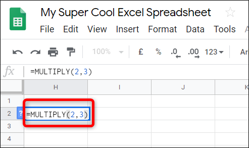
Click on an empty cell and type

        =MULTIPLY(<number1>,<number2>)
    

into the formula entry field, replacing

        <number1>
    

and

        <number2>
    

with the two integers you want to multiply.

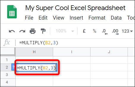
You can also use the data inside another cell. Instead of a number, type the cell number and Sheets will automatically put the integer from that cell in its place.

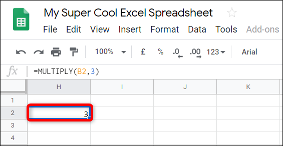
After you input the numbers or cell numbers, press the Enter key and Sheets will place the results in the cell.

Using the Multiply Operand

This method uses the multiply operand (*) to find the product of some numbers. The only difference is you're able to input more than two multiplicands, whereas the previous formula is limited to two.

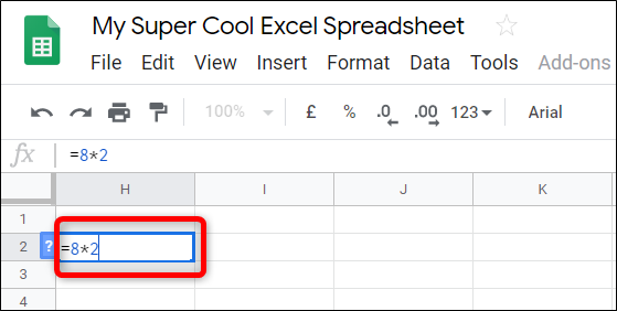
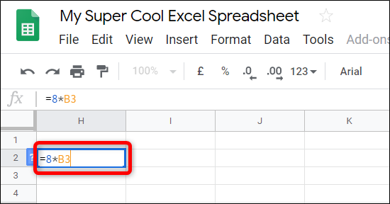
From your Google Sheets spreadsheet, click an empty cell and type

        =<number1> * <number2>
    

into the formula entry field, replacing

        <number1>
    

and

        <number2>
    

with the two integers you want to multiply.

Just like before, you can reference other cells inside the spreadsheet. Replace either number with the number of a cell that contains an integer in it.

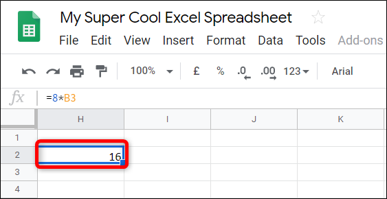
After you input the integers or cell numbers, press the Enter key and Sheets will place the results in the cell.

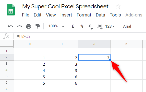
Pro tip: If you're working with a table and want to multiply the data from rows 1 and 2 into row 3, Google Sheets has a neat feature that applies the formula to the remaining cells. It fills in the remaining cells with the formula and the results. Double-click the little blue square, and, like magic, the rest of the table is filled in with the product of the two numbers.

Multiply Using ArrayFormula

This next method uses the 

        ARRAYFORMULA
    

 function to display values returned from multiple rows or columns of the same size.

From your Google Sheets spreadsheet, click an empty cell and type

        =ARRAYFORMULA(<column1> * <column2>)
    

into the formula entry field, replacing

        <column1>
    

and

        <column2>
    

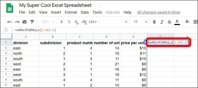
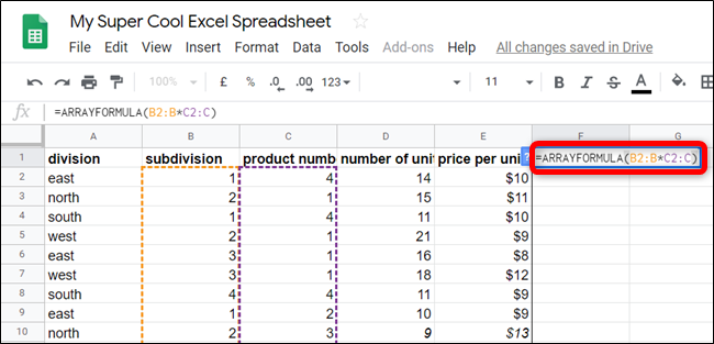
with the two columns you want to multiply. It should look something like this:

=ARRAYFORMULA(A:A*B:B)

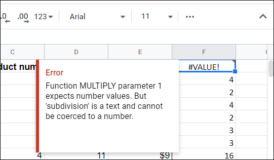
If your columns have a header in the first row, Sheets will throw an error because it expects only numbers as parameters.

Instead, you will need to start with the first cell that contains a number. For example,  instead of A:A*B:B , you would type A2:A*B2:B into the formula.

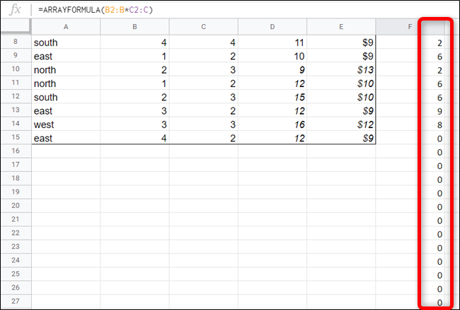
The only caveat to using the formula like this is any empty cells will use "0" in the formula. However, any other data you add to the table gets calculated dynamically, replacing each zero with the results.

If you want to limit the number of trailing zeros in your results, you should select a fixed range when you enter the formula. The new formula will look like this:

=ARRAYFORMULA(B2:B100*C2:C100)

This way, the spreadsheet uses only 100 cells as a reserve for any data you enter later. You can edit the formula and remove any unused cells by changing the 100 to a smaller number.

---

Whether you need to multiply static integers, data from two cells, or the entire contents of two columns, Google Sheets provides a couple of methods to help you calculate the product.