Filters in Google Sheets let you analyze data in your document by showing only the things you want. However, it changes how others see the document, too. Here's how to use filter views to leave each collaborator's view unchanged.
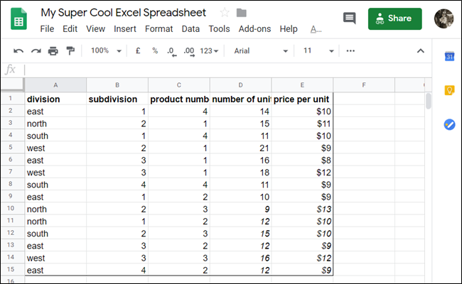
Fire up Google Sheets and open up a spreadsheet to get started.
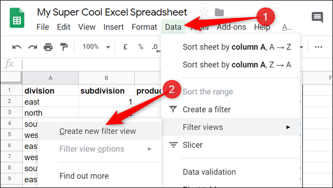
Click Data > Filter Views > Create New Filter View.
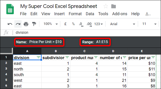
The row numbers and column letters will turn a dark gray color when activated. At this time, you should give your filter view a name to distinguish it from any other views you make in the future and check the range is correct. You can always edit both of these later if needed.
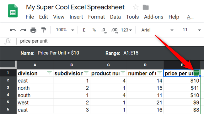
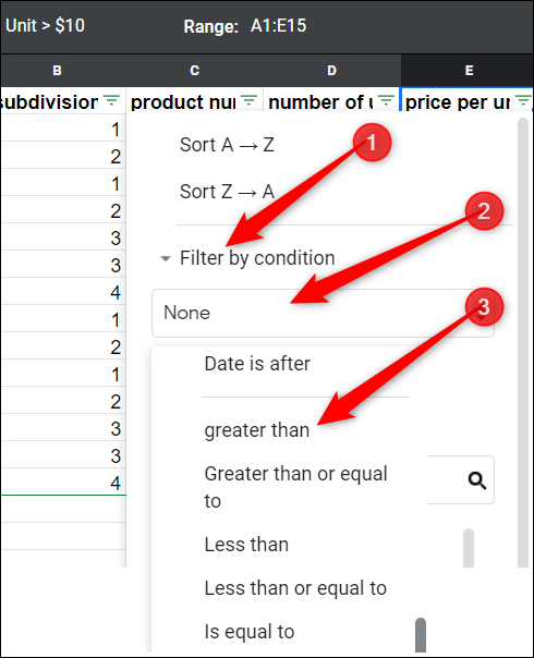
For this guide, we want to filter anything in the table that has a price per unit greater than $10. Click the filter icon in the field for "Price Per Unit."
For this next part, you can choose to filter either by values or conditions to analyze your data. "Filter by Value" offers a simple way to see data and choose specific values in the column. "Filter by Condition" gives you a much more granular approach with the option to add custom formulas to find data.
First, click "Filter by Condition" to expand the section, click the dropdown box, and then click the "Greater Than" option.
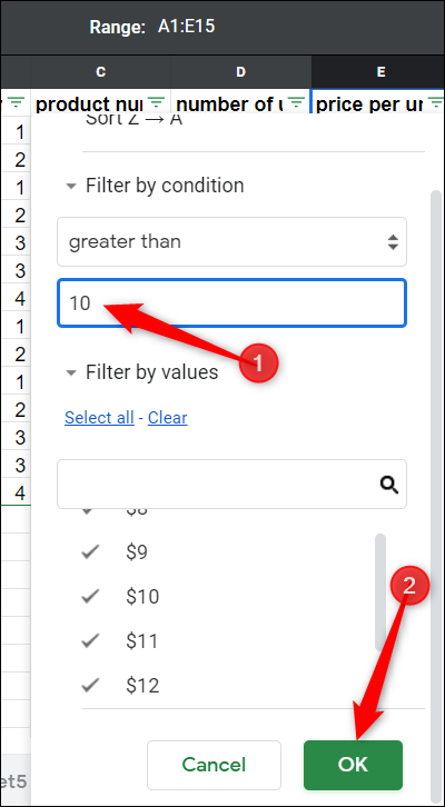
Enter the conditions for the filter and click the "OK" button.
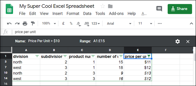
Just like that, you can now see all products that cost more than $10 per unit without disrupting the view of any other contributors.
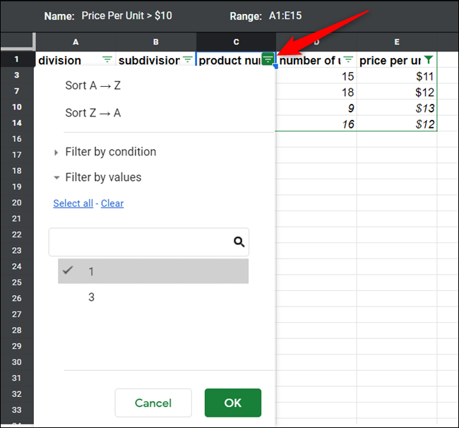
Because you can toggle only one filter at a time, you can stack filters for each column to increase your data analyzing potential. All you have to do is click on another one of the filter icons and repeat the same process.
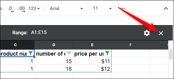
To turn all the filter views off, click the "X" in the top-right corner of the sheet.
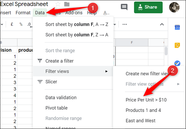
Anytime you want to turn a filtered view back on, click Data > Filter Views and then choose a filter to view.
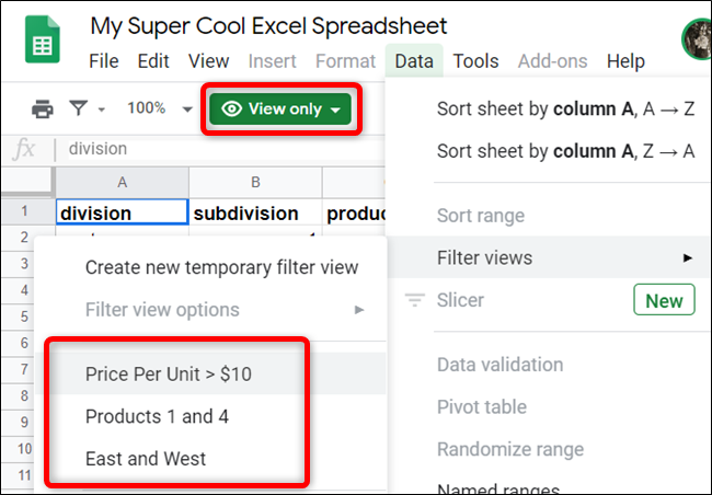
One of the great things about filter views is the ability to show filtered data without altering other collaborators' spreadsheet view. However, if anyone wants to use your filter views, they can---even people who have view-only access.
Click Data > Filter Views, and then choose one of the custom views made by other collaborators.
Although this is a very basic use of a filtered view, there seems to be no limits to its use. You can stack multiple filters and even add custom formulas to analyze and sort your data without having to disrupt other people you're working with.

