An outlier is a value that is significantly higher or lower than most of the values in your data. When using Excel to analyze data, outliers can skew the results. For example, the mean average of a data set might truly reflect your values. Excel provides a few useful functions to help manage your outliers, so let's take a look.

A Quick Example

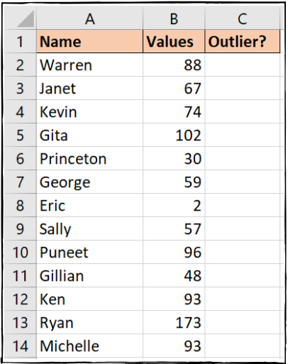
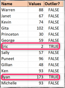
In the image below, the outliers are reasonably easy to spot---the value of two assigned to Eric and the value of 173 assigned to Ryan. In a data set like this, it's easy enough to spot and deal with those outliers manually.

In a larger set of data, that will not be the case. Being able to identify the outliers and remove them from statistical calculations is important---and that's what we'll be looking at how to do in this article.

How to Find Outliers in your Data

To find the outliers in a data set, we use the following steps:

1. Calculate the 1st and 3rd quartiles (we'll be talking about what those are in just a bit).
2. Evaluate the interquartile range (we'll also be explaining these a bit further down).
3. Return the upper and lower bounds of our data range.
4. Use these bounds to identify the outlying data points.

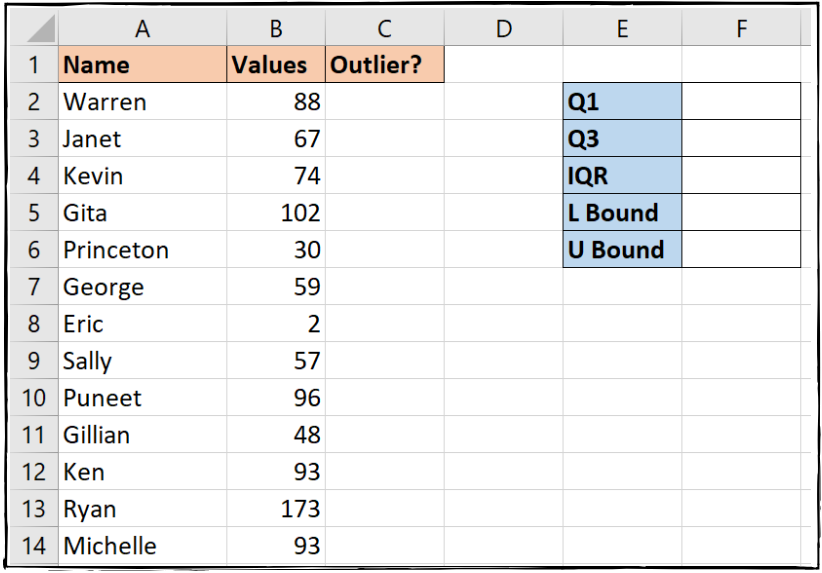
The cell range on the right of the data set seen in the image below will be used to store these values.

Let's get started.

Step One: Calculate the Quartiles

If you divide your data into quarters, each of those sets is called a quartile. The lowest 25% of numbers in the range make up the 1st quartile, the next 25% the 2nd quartile, and so on. We take this step first because the most widely-used definition of an outlier is a data point that is more than 1.5 interquartile ranges (IQRs) below the 1st quartile, and 1.5 interquartile ranges above the 3rd quartile. To determine those values, we first have to figure out what the quartiles are.

Excel provides a QUARTILE function to calculate quartiles. It requires two pieces of information: the array and the quart.

=QUARTILE(array, quart)

The array is the range of values that you are evaluating. And the quart is a number that represents the quartile you wish to return (e.g., 1 for the 1^st quartile, 2 for the 2nd quartile, and so on).

Note: In Excel 2010, Microsoft released the QUARTILE.INC and QUARTILE.EXC functions as improvements to the QUARTILE function. QUARTILE is more backward compatible when working across multiple versions of Excel.

Let's return to our example table.

To calculate the 1^st Quartile we can use the following formula in cell F2.

=QUARTILE(B2:B14,1)

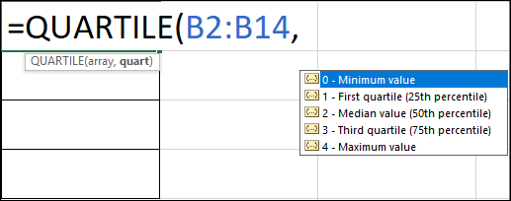
As you enter the formula, Excel provides a list of options for the quart argument.

To calculate the 3^rd quartile, we can enter a formula like the previous one in cell F3, but using a three instead of a one.

=QUARTILE(B2:B14,3)

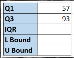
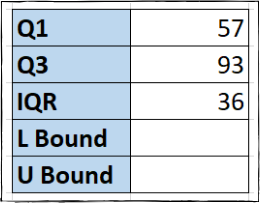
Now, we've got the quartile data points displayed in the cells.

Step Two: Evaluate the Interquartile Range

The interquartile range (or IQR) is the middle 50% of values in your data. It is calculated as the difference between the 1st quartile value and the 3rd quartile value.

We're going to use a simple formula into cell F4 that subtracts the 1^st quartile from the 3^rd quartile:

=F3-F2

Now, we can see our interquartile range displayed.

Step Three: Return the Lower and Upper Bounds

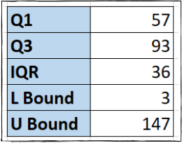
The lower and upper bounds are the smallest and largest values of the data range that we want to use. Any values smaller or larger than these bound values are the outliers.

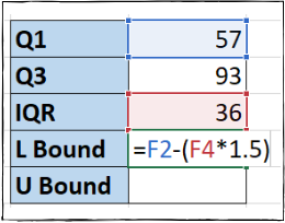
We'll calculate the lower bound limit in cell F5 by multiplying the IQR value by 1.5 and then subtracting it from the Q1 data point:

=F2-(1.5*F4)

Note: The brackets in this formula are not necessary because the multiplication part will calculate before the subtraction part, but they do make the formula easier to read.

To calculate the upper bound in cell F6, we'll multiply the IQR by 1.5 again, but this time add it to the Q3 data point:

=F3+(1.5*F4)

Step Four: Identify the Outliers

Now that we've got all our underlying data set up, it's time to identify our outlying data points---the ones that are lower than the lower bound value or higher than the upper bound value.

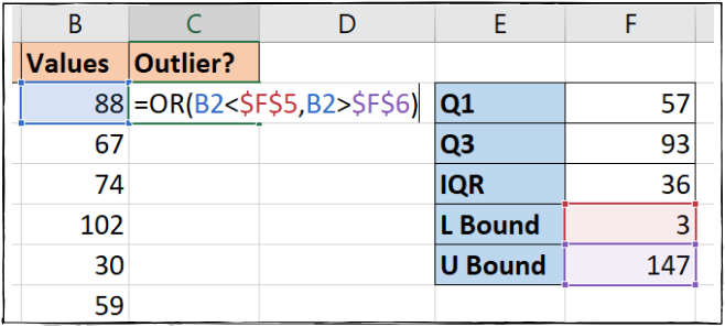
We'll use the OR function to perform this logical test and show the values that meet these criteria by entering the following formula into cell C2:

=OR(B2<$F$5,B2>$F$6)

We'll then copy that value into our C3-C14 cells. A TRUE value indicates an outlier, and as you can see, we've got two in our data.

Ignoring the Outliers when Calculating the Mean Average

Using the QUARTILE function let us calculate the IQR and work with the most widely used definition of an outlier. However, when calculating the mean average for a range of values and ignoring outliers, there is a quicker and easier function to use. This technique will not identify an outlier as before, but it will allow us to be flexible with what we might consider our outlier portion.

The function we need is called TRIMMEAN, and you can see the syntax for it below:

=TRIMMEAN(array, percent)

The array is the range of values you want to average. The percent is the percentage of data points to exclude from the top and bottom of the data set (you can enter it as a percentage or a decimal value).

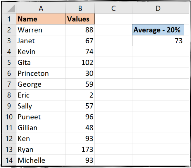
We entered the formula below into cell D3 in our example to calculate the average and exclude 20% of outliers.

=TRIMMEAN(B2:B14, 20%)

---

There you have two different functions for handling outliers. Whether you want to identify them for some reporting needs or exclude them from calculations such as averages, Excel has a function to fit your needs.