In a recent article, we introduced the Excel function called VLOOKUP and explained how it could be used to retrieve information from a database into a cell in a local worksheet. In that article we mentioned that there were two uses for VLOOKUP, and only one of them dealt with querying databases. In this article, the second and final in the VLOOKUP series, we examine this other, lesser known use for the VLOOKUP function. If you haven't already done so, please read the first VLOOKUP article - this article will assume that many of the concepts explained in that article are already known to the reader. When working with databases, VLOOKUP is passed a "unique identifier" that serves to identify which data record we wish to find in the database (e.g. a product code or customer ID). This unique identifier must exist in the database, otherwise VLOOKUP returns us an error. In this article, we will examine a way of using VLOOKUP where the identifier doesn't need to exist in the database at all. It's almost as if VLOOKUP can adopt a "near enough is good enough" approach to returning the data we're looking for. In certain circumstances, this is exactly what we need. We will illustrate this article with a real-world example - that of calculating the commissions that are generated on a set of sales figures. We will start with a very simple scenario, and then progressively make it more complex, until the only rational solution to the problem is to use VLOOKUP. The initial scenario in our fictitious company works like this: If a salesperson creates more than $30,000 worth of sales in a given year, the commission they earn on those sales is 30%. Otherwise their commission is only 20%. So far this is a pretty simple worksheet: To use this worksheet, the salesperson enters their sales figures in cell B1, and the formula in cell B2 calculates the correct commission rate they are entitled to receive, which is used in cell B3 to calculate the total commission that the salesperson is owed (which is a simple multiplication of B1 and B2). The cell B2 contains the only interesting part of this worksheet - the formula for deciding which commission rate to use: the one below the threshold of $30,000, or the one above the threshold. This formula makes use of the Excel function called IF. For those readers that are not familiar with IF, it works like this:
IF(condition,value if true,value if false)
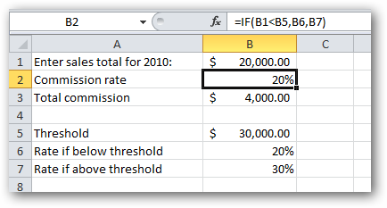
Where the condition is an expression that evaluates to either true or false. In the example above, the condition is the expression B1<B5, which can be read as "Is B1 less than B5?", or, put another way, "Are the total sales less than the threshold". If the answer to this question is "yes" (true), then we use the value if true parameter of the function, namely B6 in this case - the commission rate if the sales total was below the threshold. If the answer to the question is "no" (false), then we use the value if false parameter of the function, namely B7 in this case - the commission rate if the sales total was above the threshold. As you can see, using a sales total of $20,000 gives us a commission rate of 20% in cell B2. If we enter a value of $40,000, we get a different commission rate:

So our spreadsheet is working. Let's make it more complex. Let's introduce a second threshold: If the salesperson earns more than $40,000, then their commission rate increases to 40%:

Easy enough to understand in the real world, but in cell B2 our formula is getting more complex. If you look closely at the formula, you'll see that the third parameter of the original IF function (the value if false) is now an entire IF function in its own right. This is called a nested function (a function within a function). It's perfectly valid in Excel (it even works!), but it's harder to read and understand. We're not going to go into the nuts and bolts of how and why this works, nor will we examine the nuances of nested functions. This is a tutorial on VLOOKUP, not on Excel in general. Anyway, it gets worse! What about when we decide that if they earn more than $50,000 then they're entitled to 50% commission, and if they earn more than $60,000 then they're entitled to 60% commission?

Now the formula in cell B2, while correct, has become virtually unreadable. No-one should have to write formulae where the functions are nested four levels deep! Surely there must be a simpler way? There certainly is. VLOOKUP to the rescue! Let's redesign the worksheet a bit. We'll keep all the same figures, but organize it in a new way, a more tabular way:

Take a moment and verify for yourself that the new Rate Table works exactly the same as the series of thresholds above. Conceptually, what we're about to do is use VLOOKUP to look up the salesperson's sales total (from B1) in the rate table and return to us the corresponding commission rate. Note that the salesperson may have indeed created sales that are not one of the five values in the rate table ($0, $30,000, $40,000, $50,000 or $60,000). They may have created sales of $34,988. It's important to note that $34,988 does not appear in the rate table. Let's see if VLOOKUP can solve our problem anyway... We select cell B2 (the location we want to put our formula), and then insert the VLOOKUP function from the Formulas tab:

The Function Arguments box for VLOOKUP appears. We fill in the arguments (parameters) one by one, starting with the Lookup_value, which is, in this case, the sales total from cell B1. We place the cursor in the Lookup_value field and then click once on cell B1:

Next we need to specify to VLOOKUP what table to lookup this data in. In this example, it's the rate table, of course. We place the cursor in the Table_array field, and then highlight the entire rate table - excluding the headings:

Next we must specify which column in the table contains the information we want our formula to return to us. In this case we want the commission rate, which is found in the second column in the table, so we therefore enter a 2 into the Col_index_num field:

Finally we enter a value in the Range_lookup field. Important: It is the use of this field that differentiates the two ways of using VLOOKUP. To use VLOOKUP with a database, this final parameter, Range_lookup, must always be set to FALSE, but with this other use of VLOOKUP, we must either leave it blank or enter a value of TRUE. When using VLOOKUP, it is vital that you make the correct choice for this final parameter. To be explicit, we will enter a value of true in the Range_lookup field. It would also be fine to leave it blank, as this is the default value:

We have completed all the parameters. We now click the OK button, and Excel builds our VLOOKUP formula for us:

If we experiment with a few different sales total amounts, we can satisfy ourselves that the formula is working. Conclusion In the "database" version of VLOOKUP, where the Range_lookup parameter is FALSE, the value passed in the first parameter (Lookup_value) must be present in the database. In other words, we're looking for an exact match. But in this other use of VLOOKUP, we are not necessarily looking for an exact match. In this case, "near enough is good enough". But what do we mean by "near enough"? Let's use an example: When searching for a commission rate on a sales total of $34,988, our VLOOKUP formula will return us a value of 30%, which is the correct answer. Why did it choose the row in the table containing 30% ? What, in fact, does "near enough" mean in this case? Let's be precise:
When Range_lookup is set to TRUE (or omitted), VLOOKUP will look in column 1 and match the highest value that is not greater than the Lookup_value parameter.
It's also important to note that for this system to work, the table must be sorted in ascending order on column 1! If you would like to practice with VLOOKUP, the sample file illustrated in this article can be downloaded from here.