When working on an Excel worksheet, you may find yourself setting up different display settings at different times, such as zoom level or window position and size. The Custom Views feature allows you to set up and save different views to quickly switch among them.
For example, you may want to zoom in on the worksheet temporarily to see more details, or hide parts of the Excel interface to maximize your workspace (in addition to hiding the ribbon). You can set up a different view for each worksheet and save each view. The following settings are included in custom views: the zoom level, the current cell selection, column widths and row heights, display settings on the Advanced tab of the Excel Options dialog box, the current size and position of the document window, the window pane arrangement (including frozen rows and columns), and optionally print settings (including page setup) and hidden columns and rows.
Before setting up any custom views, it’s a good idea to save the current normal view as a custom view so you can easily revert back to it. To set the current view as the normal view, click the “View” tab.

In the Workbook Views section, click “Custom Views” or hold Alt and press W, then C on your keyboard.

On the Custom Views dialog box, click “Add”

Type a unique name for the view in the “Name” box. Since this is our normal view, we named it “Normal 100%”. Either check or uncheck the “Print settings” and “Hidden rows, columns and filter settings” boxes depending on what you want to include in the view. Click “OK”.

Now, we’ll create a custom view. As an example, we’re going to create a view with a 150% zoom and the Formula Bar and Headings hidden, so we can read our spreadsheet easily and have a bit more room on the worksheet. Set up the view the way you want it and then click “Custom Views” in the Workbook Views section on the View tab.

Click “Add” on the Custom Views dialog box.

Enter a unique name for your custom view and check or uncheck the boxes under Include in view as desired.

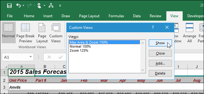
To switch views, click “Custom Views” in the Workbook Views section on the View tab, or hold Alt and press W, then C on your keyboard. Click on the view you want and click “Show”. You can also double-click the name of the view you want to show.

Custom views are only available in the workbook in which you create them, and they are saved as part of the workbook. They are also worksheet-specific, meaning that a custom view only applies to the worksheet that was active when you created the custom view. When you choose a custom view to show for a worksheet that is not currently active, Excel activates that worksheet and applies the view. So, you must create custom views for each worksheet in each workbook separately and be sure to save your workbook with your custom views.